Hey everyone!
Today I’m going to talk about a simple but very powerful tool in Excel: Conditional Formatting.
What is Conditional Formatting?
Conditional Formatting is a simple way that you can format your data based on conditions. This opens up a wide range of beneficial use cases, for example:
- Find areas to focus attention – Highlight in red any Sales data that falls below a target
- Project or task tracking – Highlight in green any project or task that is complete
- Find data anomalies or issues – Highlight in red any blank or 0 cells where there shouldn’t be
Example – Project Task Tracking
Say we have a basic project tracking worksheet, like this:

Download the file here:
Say we’re the project manager for all of these projects, and we want to do the following:
- Highlight in green the whole row for any project that is 100% complete
- Highlight in red any project that is past due but not 100% complete
But first, let’s cover the basics:
Creating a Conditional Formatting Rule
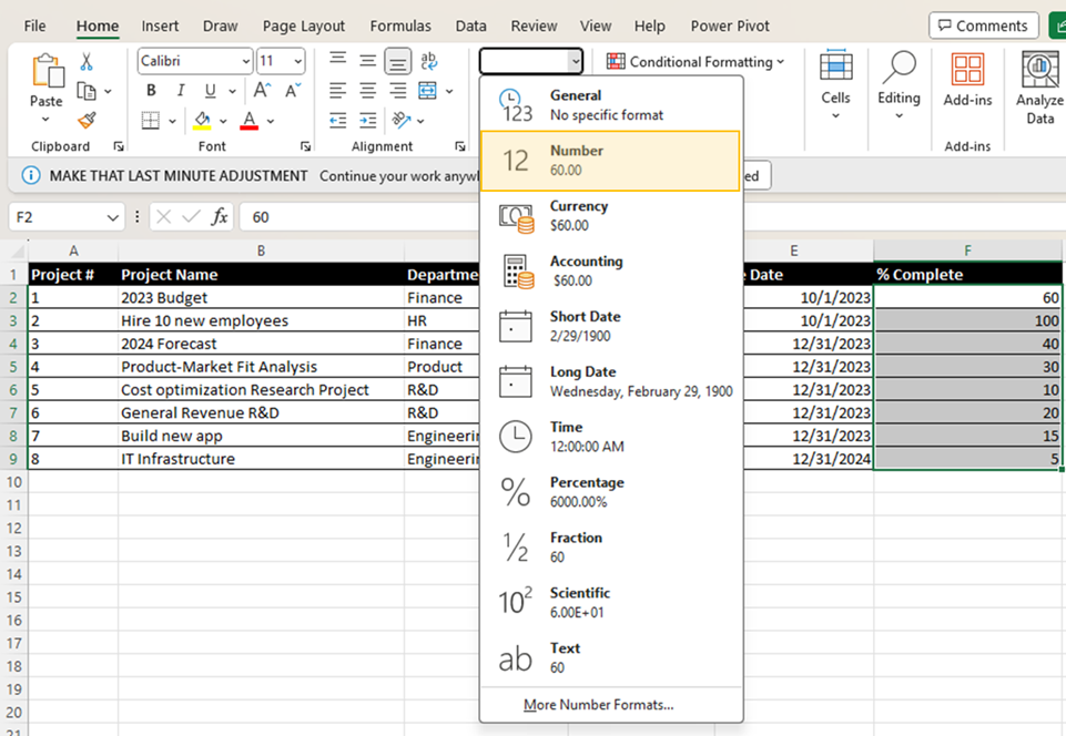
As a prerequisite, let’s change our values in the “% Complete” to “Number” formatting. To do this, highlight the range F2:F9, click the formatting drop-down on the Home tab and select “Number”:
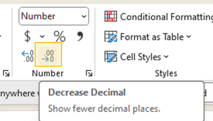
This is great, but it will add two decimals to our percentages that we don’t want. To remove these, leave the range highlighted and click on “Decrease Decimal” twice:
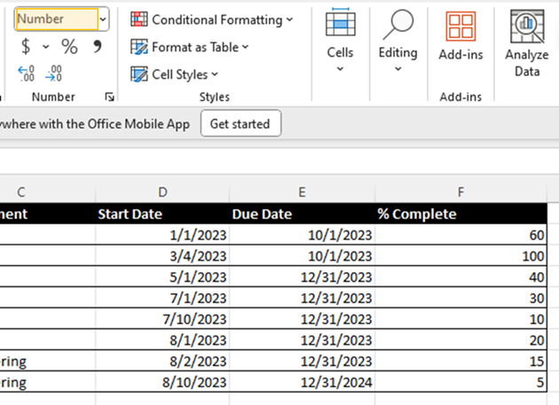
So now our data will look like before, but this column is all in “Number” format now. This is needed to make sure the conditional formatting rules work right.
Ok now let’s just create a basic Conditional Formatting rule:
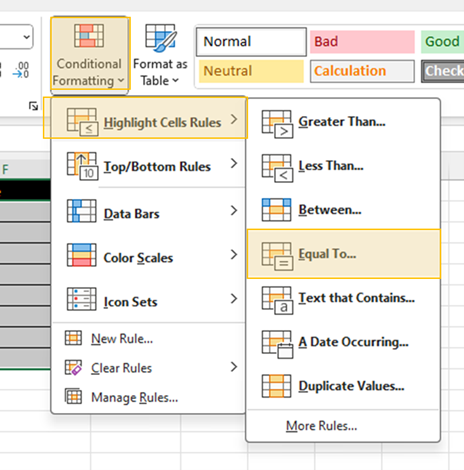
Highlight your data (or Ctrl + A) and click on “Conditional Formatting” -> “Highlight Cells Rules” -> “Equal To…”:
A dialog box will appear:
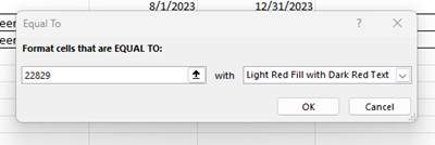
Enter 100 in the box and select “Green Fill with Dark Green Text” from the drop-down. Click “OK”:

Here’s what we get:

Pretty cool, right?
This works fine for many use cases, but say we want to highlight the whole row, not just the one cell where the value appears. This will make the row stand out much more.
Clearing Conditional Formatting Rules
To start over, let’s go ahead and clear the formatting rule we created.
Go to “Conditional Formatting” -> “Clear Rules” -> “Clear Rules from Entire Sheet”:
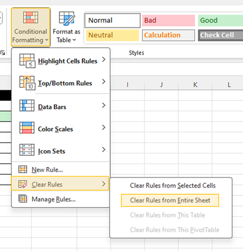
This will remove the conditional formatting rule we created, so we’re starting over.
Highlighting the whole row based on a cell value
Creating a New Rule
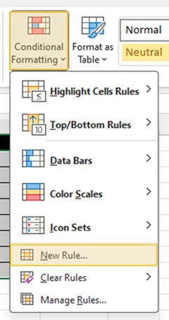
Now, let’s do this again. This time, we’re going to highlight the data and go to “Conditional Formatting” -> “New Rule…”. This will allow us to create a more custom rule, rather than the simple default one we did above.
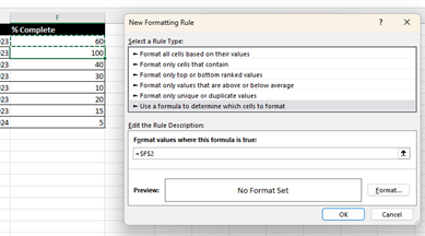
In the dialog box that opens, select “Use a formula to determine which cells to format”:

In the formula bar, enter the following:
=$F1=100
Another way to do this step-by-step is:
- Enter “=” in the formula bar

2. Click on the F2 cell
3. Hit F4 on your keyboard twice. This adds the $ before the F, which “locks” the column (more explanation below).

4. Enter “=100”

How the Formula Works
This formula compares each cell in the F column to the value 100, but since the formatting rule applies to the entire range A2-F9, it will highlight the entire row, not just the F column.
The secret here is to use the $ next to F: this “locks” the column to F for the purpose of doing the comparison. So, if the value 100 appears in any other column, it will not be highlighted because I’m only comparing column F.
That’s it for the formula.
Finishing Up
Now, let’s set the formatting: click on “Format…”
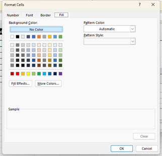
Navigate to the “Fill” tab and select your favorite shade of green (or any color you like), and click “OK”.

Pretty cool!
Highlighting the whole row based on two conditions
Now that we’ve learned how to highlight the whole row based on a condition, let’s try the second use case we mentioned in the beginning:
Highlight in green the whole row for any project that is 100% complete- Highlight in red any project that is past due but not 100% complete
Breaking this down, we see that this has two conditions that we need to apply, whereas our first use case only had one.
There’s several ways to tackle this, but I’m going to use the AND() function.
Setting up the rule
First, we follow the same steps as before:
- Highlight the data and go to “Conditional Formatting” -> “New Rule…”.

2. In the dialog box that opens, select “Use a formula to determine which cells to format”:
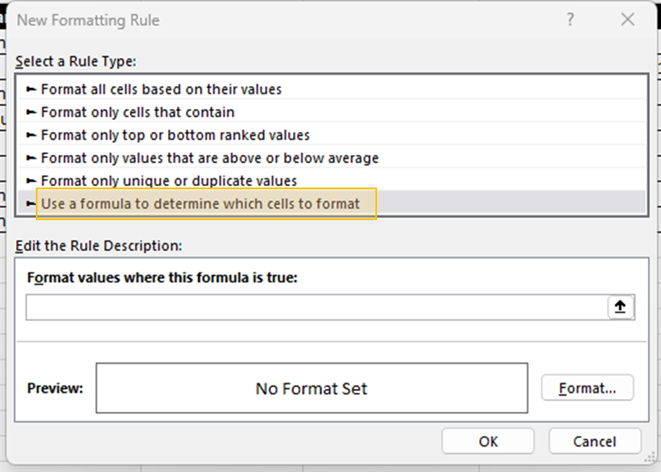
Here is where we enter the formula:
=AND($F2<100,$E2<TODAY())
Click on “Format…”

Navigate to the “Fill” tab and now let’s pick a shade of red (since we’re highlighting projects that are past due), and click “OK”.

As you can see, the first row is a project that is past due (was due on 10/1/23 but today is 11/4/23) and is NOT 100% complete. Nice!
Understanding the Formula
Let’s break down the formula to make sure we understand:
=AND($F2<100,$E2<TODAY())
The AND() function takes two or more arguments (inputs), evaluates each one to TRUE or FALSE, and it will return TRUE only if both conditions are true.
So in this case, the full row will only be highlighted if BOTH the below conditions are true:
- The numeric value in column F is less than 100 (this is the $F2<100 portion)
- The date value in column E is before today’s date (this is the $E2<TODAY() portion)
Together, these two conditions give us what we want – only highlight the row in red when BOTH the project is less than 100% complete AND the due date has already past.
Bonus: Filter by Color
The conditional color highlighting we just learned is great, but what if we have a lot of data that we don’t want to scroll through to find every instance of green or red?
Here’s where filtering by color comes in.
To filter by color,
- Click in any column of the first (“header”) row of the data

2. Go to the “Data” tab in the toolbar and click on “Filter”

3. In any column (since the whole row is highlighted), click on the drop-down that appeared, hover over “Filter by color” and select which color you’d like to filter by.
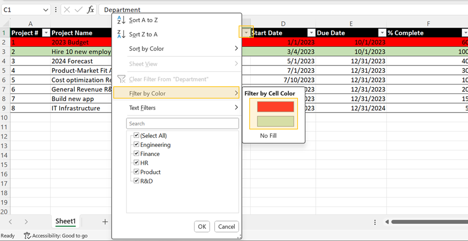
Now you’ll only see rows that are the color you selected, for example red:

That’s it for today, let me know what you think in the comments below!